Polynomial and Non-Linear Regression

2025-11-02

Linear regression is great when your data follows a straight line. But what happens when your relationship is curved? When house prices don’t increase linearly with size, or when population growth accelerates exponentially? That’s where polynomial and non-linear regression come in.

This article shows you how to move beyond straight lines to model the curves and patterns you see in real data.

The Problem with Straight Lines

Linear regression assumes relationships are linear. But many real-world phenomena are inherently curved:

• Population growth follows exponential curves
• Drug effectiveness plateaus at high doses
• Learning curves show diminishing returns
• Physical phenomena follow power laws or logarithmic patterns

When you force a straight line through curved data, you get poor predictions and miss the true relationship.

import numpy as np
import matplotlib.pyplot as plt
from sklearn.linear_model import LinearRegression
from sklearn.metrics import r2_score

# Generate curved data (quadratic relationship)
np.random.seed(42)
X = np.linspace(0, 10, 100).reshape(-1, 1)
y = 2 * X.squeeze()**2 - 5 * X.squeeze() + 3 + np.random.randn(100) * 10

# Try linear regression
linear_model = LinearRegression()
linear_model.fit(X, y)
linear_pred = linear_model.predict(X)

plt.figure(figsize=(10, 6))
plt.scatter(X, y, alpha=0.5, label='Data')
plt.plot(X, linear_pred, 'r-', linewidth=2, label='Linear fit')
plt.xlabel('X')
plt.ylabel('y')
plt.title(f'Linear Regression on Curved Data (R² = {r2_score(y, linear_pred):.3f})')
plt.legend()
plt.show()

# Poor R² score shows linear model doesn't fit well
print(f"Linear model R²: {r2_score(y, linear_pred):.3f}")

Output:

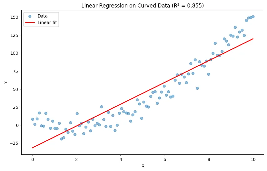
Linear model R²: 0.855

What is Polynomial Regression?

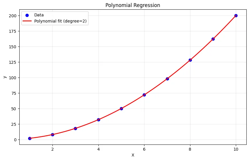
Polynomial regression extends linear regression by adding polynomial terms (squared, cubed, etc.) of your features. The key insight: it’s still linear in the coefficients, just non-linear in the features.

The Math

Instead of:

We use:

Where $n$ is the degree of the polynomial.

Why It Works

Even though the relationship between $x$ and $y$ is non-linear, the relationship between the coefficients ($\beta$ values) and $y$ remains linear. This means we can still use linear regression techniques under the hood.

Python Implementation

from sklearn.preprocessing import PolynomialFeatures
from sklearn.linear_model import LinearRegression
import numpy as np

# Sample data: curved relationship
X = np.array([1, 2, 3, 4, 5, 6, 7, 8, 9, 10]).reshape(-1, 1)
y = np.array([2, 8, 18, 32, 50, 72, 98, 128, 162, 200])

# Create polynomial features and fit model
poly_features = PolynomialFeatures(degree=2, include_bias=False)
X_poly = poly_features.fit_transform(X)

# See what polynomial features look like
print("Original features:", X[:3].flatten())
print("Polynomial features:", X_poly[:3])
# Original: [1, 2, 3]
# Polynomial: [[1, 1], [2, 4], [3, 9]]  # [x, x²]

# Fit polynomial regression
poly_model = LinearRegression()
poly_model.fit(X_poly, y)

# Make predictions
poly_pred = poly_model.predict(X_poly)

# Compare results
print(f"\nPolynomial model R²: {r2_score(y, poly_pred):.3f}")
print(f"Coefficients: {poly_model.coef_}")
print(f"Intercept: {poly_model.intercept_:.2f}")

# Plot results
X_plot = np.linspace(1, 10, 100).reshape(-1, 1)
X_plot_poly = poly_features.transform(X_plot)
y_plot = poly_model.predict(X_plot_poly)

plt.figure(figsize=(10, 6))
plt.scatter(X, y, color='blue', s=50, label='Data')
plt.plot(X_plot, y_plot, 'r-', linewidth=2, label='Polynomial fit (degree=2)')
plt.xlabel('X')
plt.ylabel('y')
plt.title('Polynomial Regression')
plt.legend()
plt.grid(True, alpha=0.3)
plt.show()

Output:

Original features: [1 2 3]
Polynomial features: [[1. 1.]
 [2. 4.]
 [3. 9.]]

Polynomial model R²: 1.000
Coefficients: [1.0311238e-15 2.0000000e+00]
Intercept: 0.00

Using Pipeline for Cleaner Code

from sklearn.pipeline import make_pipeline

# Create pipeline: polynomial features → linear regression
degree = 2
poly_model = make_pipeline(
    PolynomialFeatures(degree=degree),
    LinearRegression()
)

# Fit and predict in one go
poly_model.fit(X, y)
predictions = poly_model.predict(X)

print(f"R² Score: {r2_score(y, predictions):.3f}")

Output:

R² Score: 1.000

Choosing the Right Polynomial Degree

The degree of your polynomial is critical. Too low and you underfit; too high and you overfit.

Comparing Different Degrees

import matplotlib.pyplot as plt
from sklearn.metrics import mean_squared_error

# Generate data with noise
np.random.seed(42)
X = np.linspace(0, 10, 50).reshape(-1, 1)
y = 2 * X.squeeze()**2 - 5 * X.squeeze() + 3 + np.random.randn(50) * 10

# Try different polynomial degrees
degrees = [1, 2, 3, 5, 10]
plt.figure(figsize=(15, 10))

for idx, degree in enumerate(degrees, 1):
    # Fit model
    model = make_pipeline(
        PolynomialFeatures(degree=degree),
        LinearRegression()
    )
    model.fit(X, y)
    
    # Create smooth line for plotting
    X_plot = np.linspace(0, 10, 200).reshape(-1, 1)
    y_plot = model.predict(X_plot)
    
    # Calculate metrics
    y_pred = model.predict(X)
    r2 = r2_score(y, y_pred)
    mse = mean_squared_error(y, y_pred)
    
    # Plot
    plt.subplot(2, 3, idx)
    plt.scatter(X, y, alpha=0.5, s=20)
    plt.plot(X_plot, y_plot, 'r-', linewidth=2)
    plt.xlabel('X')
    plt.ylabel('y')
    plt.title(f'Degree {degree}\nR²={r2:.3f}, MSE={mse:.1f}')
    plt.ylim(-50, 250)

plt.tight_layout()
plt.show()

Output:

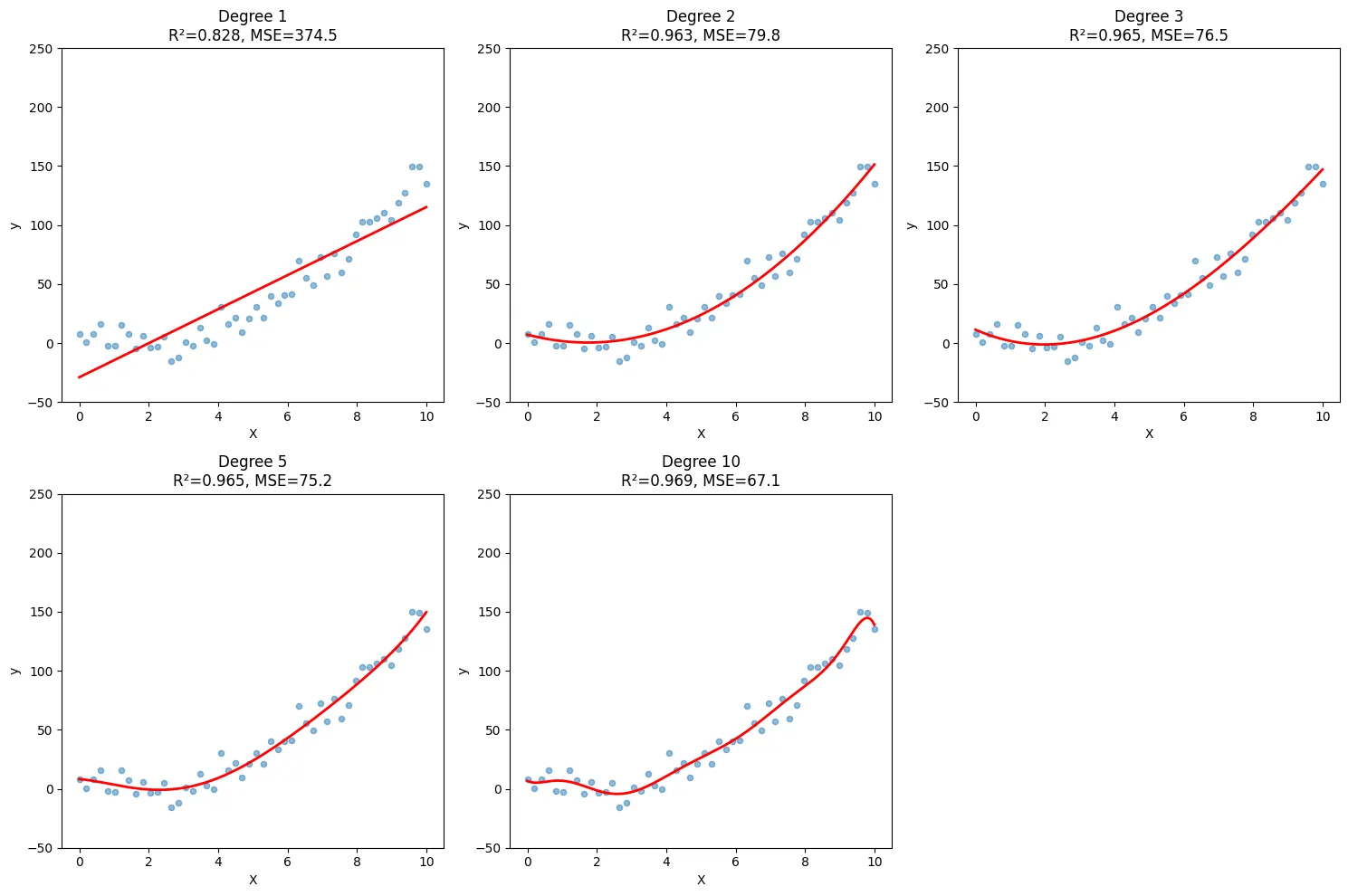
What You’ll See

• Degree 1 (linear): Underfits - misses the curve
• Degree 2-3: Good fit - captures the pattern
• Degree 10+: Overfits - wild fluctuations between points

Using Cross-Validation to Choose Degree

from sklearn.model_selection import cross_val_score

# Test different degrees with cross-validation
degrees = range(1, 11)
cv_scores = []

for degree in degrees:
    model = make_pipeline(
        PolynomialFeatures(degree=degree),
        LinearRegression()
    )
    # Use negative MSE (sklearn convention)
    scores = cross_val_score(model, X, y, cv=5, 
                            scoring='neg_mean_squared_error')
    cv_scores.append(-scores.mean())

# Plot cross-validation scores
plt.figure(figsize=(10, 6))
plt.plot(degrees, cv_scores, marker='o', linewidth=2)
plt.xlabel('Polynomial Degree')
plt.ylabel('Cross-Validation MSE')
plt.title('Finding Optimal Polynomial Degree')
plt.grid(True, alpha=0.3)
plt.show()

# Best degree has lowest CV error
best_degree = degrees[np.argmin(cv_scores)]
print(f"Optimal polynomial degree: {best_degree}")

Output:

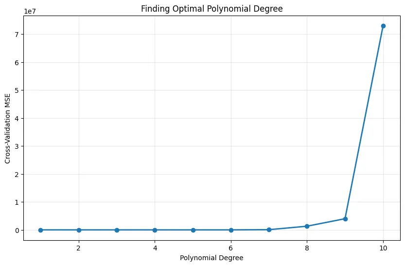
Optimal polynomial degree: 2

Multiple Features with Polynomial Terms

Polynomial regression also works with multiple features, creating interaction terms.

from sklearn.preprocessing import PolynomialFeatures
import pandas as pd

# Sample data: house price with two features
data = pd.DataFrame({
    'size': [1000, 1500, 2000, 2500, 3000],
    'age': [5, 10, 2, 15, 8],
    'price': [200000, 280000, 420000, 380000, 550000]
})

X = data[['size', 'age']]
y = data['price']

# Create polynomial features (degree=2)
poly = PolynomialFeatures(degree=2, include_bias=False)
X_poly = poly.fit_transform(X)

# See what features were created
feature_names = poly.get_feature_names_out(['size', 'age'])
print("Created features:", feature_names)
# Output: ['size', 'age', 'size^2', 'size age', 'age^2']

# Fit model
model = LinearRegression()
model.fit(X_poly, y)

# Show coefficients
coef_df = pd.DataFrame({
    'feature': feature_names,
    'coefficient': model.coef_
})
print("\nCoefficients:")
print(coef_df)

Output:

Created features: ['size' 'age' 'size^2' 'size age' 'age^2']

Coefficients:
    feature  coefficient
0      size   511.279986
1       age  1059.217940
2    size^2    -0.109939
3  size age    16.405703
4     age^2 -2767.596262

Key Points About Multiple Features

• Interaction terms: $x_1 \cdot x_2$ captures how features interact
• Feature explosion: 10 features with degree 3 creates hundreds of features
• Multicollinearity: High-degree polynomials create correlated features
• Regularization helps: Use Ridge or Lasso to handle many polynomial features

Beyond Polynomials: Other Non-Linear Models

Not all curves are polynomial. Sometimes you need exponential, logarithmic, or other transformations.

Exponential Relationships

import numpy as np
import matplotlib.pyplot as plt
from sklearn.linear_model import LinearRegression

# Generate exponential data: y = a * e^(bx)
np.random.seed(42)  # for reproducibility
X = np.linspace(0, 5, 50).reshape(-1, 1)

# Add noise in log space (multiplicative in original space)
y_true = 2 * np.exp(0.5 * X.squeeze())
y = y_true * np.exp(np.random.randn(50) * 0.2)  # Multiplicative noise

# Now y is always positive, so log(y) is safe
y_log = np.log(y)

# Fit linear model on transformed data
model = LinearRegression()
model.fit(X, y_log)

# Transform predictions back
y_pred_log = model.predict(X)
y_pred = np.exp(y_pred_log)

plt.figure(figsize=(12, 5))

plt.subplot(1, 2, 1)
plt.scatter(X, y_log, alpha=0.5)
plt.plot(X, y_pred_log, 'r-', linewidth=2)
plt.xlabel('X')
plt.ylabel('log(y)')
plt.title('Linear in Log Space')
plt.grid(True, alpha=0.3)

plt.subplot(1, 2, 2)
plt.scatter(X, y, alpha=0.5)
plt.plot(X, y_pred, 'r-', linewidth=2)
plt.xlabel('X')
plt.ylabel('y')
plt.title('Exponential in Original Space')
plt.grid(True, alpha=0.3)

plt.tight_layout()
plt.show()

print(f"Exponential model: y = {np.exp(model.intercept_):.2f} * e^({model.coef_[0]:.2f}x)")

Output:

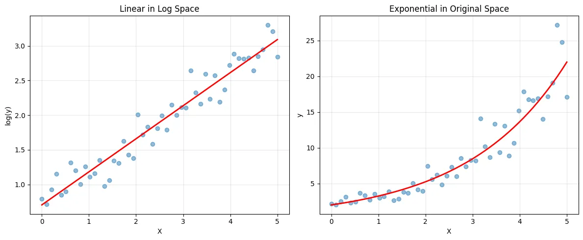
Exponential model: y = 2.03 * e^(0.48x)

Logarithmic Relationships

# Generate logarithmic data: y = a + b * log(x)
X = np.linspace(1, 100, 50).reshape(-1, 1)
y = 5 + 3 * np.log(X.squeeze()) + np.random.randn(50) * 2

# Transform features: use log(x)
X_log = np.log(X)

# Fit linear model
model = LinearRegression()
model.fit(X_log, y)
y_pred = model.predict(X_log)

plt.figure(figsize=(10, 6))
plt.scatter(X, y, alpha=0.5, label='Data')
plt.plot(X, y_pred, 'r-', linewidth=2, label='Logarithmic fit')
plt.xlabel('X')
plt.ylabel('y')
plt.title('Logarithmic Regression')
plt.legend()
plt.show()

print(f"Logarithmic model: y = {model.intercept_:.2f} + {model.coef_[0]:.2f} * log(x)")

Output:

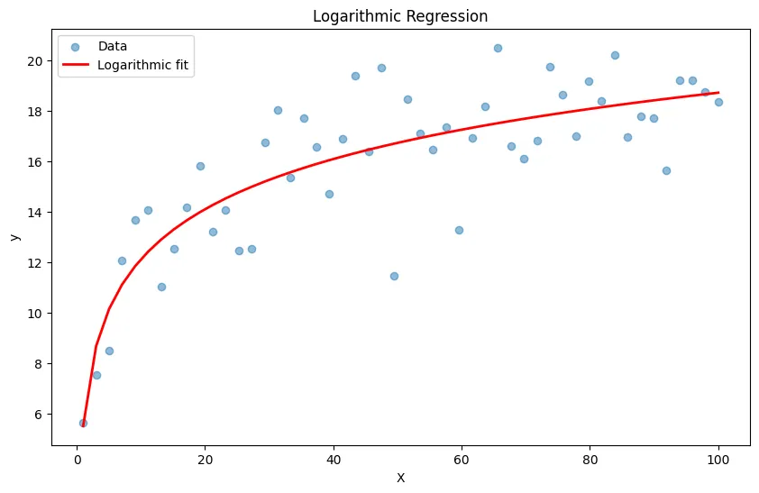
Logarithmic model: y = 5.52 + 2.87 * log(x)

Power Law Relationships

import numpy as np
import matplotlib.pyplot as plt
from sklearn.linear_model import LinearRegression

# Generate power law data: y = a * x^b
np.random.seed(42)
X = np.linspace(1, 10, 50).reshape(-1, 1)

# Use multiplicative noise
y_true = 2 * X.squeeze()**1.5
y = y_true * np.exp(np.random.randn(50) * 0.15)  # Multiplicative noise

# Transform to linear: log(y) = log(a) + b*log(x)
X_log = np.log(X)
y_log = np.log(y)

model = LinearRegression()
model.fit(X_log, y_log)

# Transform predictions back
y_pred_log = model.predict(X_log)
y_pred = np.exp(y_pred_log)

plt.figure(figsize=(10, 6))
plt.scatter(X, y, alpha=0.5, label='Data')
plt.plot(X, y_pred, 'r-', linewidth=2, label='Power law fit')
plt.xlabel('X')
plt.ylabel('y')
plt.title('Power Law Regression')
plt.legend()
plt.grid(True, alpha=0.3)
plt.show()

power = model.coef_[0]
constant = np.exp(model.intercept_)
print(f"Power law model: y = {constant:.2f} * x^{power:.2f}")

Output:

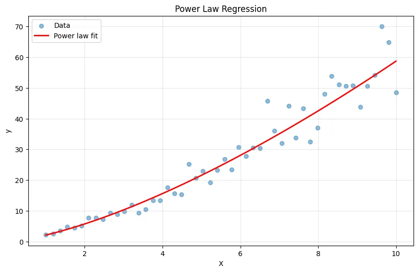
Power law model: y = 2.10 * x^1.45

Common Pitfalls and How to Avoid Them

1. Overfitting with High-Degree Polynomials

Problem: High-degree polynomials fit training data perfectly but fail on new data.

from sklearn.model_selection import train_test_split

# Generate data
np.random.seed(42)
X = np.linspace(0, 10, 30).reshape(-1, 1)
y = 2 * X.squeeze()**2 - 5 * X.squeeze() + 3 + np.random.randn(30) * 10

# Split data
X_train, X_test, y_train, y_test = train_test_split(X, y, test_size=0.3, random_state=42)

# Compare degree 2 vs degree 10
for degree in [2, 10]:
    model = make_pipeline(
        PolynomialFeatures(degree=degree),
        LinearRegression()
    )
    model.fit(X_train, y_train)
    
    train_score = model.score(X_train, y_train)
    test_score = model.score(X_test, y_test)
    
    print(f"\nDegree {degree}:")
    print(f"  Train R²: {train_score:.3f}")
    print(f"  Test R²: {test_score:.3f}")
    print(f"  Overfit gap: {train_score - test_score:.3f}")

Output:

Degree 2:
  Train R²: 0.961
  Test R²: 0.983
  Overfit gap: -0.023

Degree 10:
  Train R²: 0.981
  Test R²: 0.809
  Overfit gap: 0.172

Solution: Use cross-validation, regularization (Ridge/Lasso), or limit polynomial degree.

2. Feature Scaling Becomes Critical

Problem: Polynomial features create huge value ranges that can cause numerical issues.

from sklearn.preprocessing import StandardScaler

# Data with different scales
X = np.array([[1000, 2], [1500, 3], [2000, 4]]).astype(float)
y = np.array([200000, 300000, 400000])

# Without scaling
poly_model_unscaled = make_pipeline(
    PolynomialFeatures(degree=2),
    LinearRegression()
)
poly_model_unscaled.fit(X, y)

# With scaling
poly_model_scaled = make_pipeline(
    StandardScaler(),
    PolynomialFeatures(degree=2),
    LinearRegression()
)
poly_model_scaled.fit(X, y)

print("Unscaled coefficients:", poly_model_unscaled.named_steps['linearregression'].coef_)
print("\nScaled coefficients:", poly_model_scaled.named_steps['linearregression'].coef_)

Output:

Unscaled coefficients: [ 6.98748143e-11  1.99999200e+02  3.99998400e-01 -1.76247905e-15
  8.97490957e-13  1.49702877e-15]

Scaled coefficients: [ 7.27595761e-12  4.08248290e+04  4.08248290e+04 -1.81898940e-12
  5.45696821e-12 -1.81898940e-12]

Solution: Always scale features before creating polynomial terms, especially with high degrees.

3. Extrapolation Danger

Problem: Polynomial models go wild outside the training data range.

# Train on limited range
X_train = np.linspace(0, 5, 30).reshape(-1, 1)
y_train = 2 * X_train.squeeze()**2 + 10 + np.random.randn(30) * 5

# Fit high-degree polynomial
model = make_pipeline(
    PolynomialFeatures(degree=5),
    LinearRegression()
)
model.fit(X_train, y_train)

# Try to extrapolate
X_extended = np.linspace(-2, 10, 100).reshape(-1, 1)
y_extended = model.predict(X_extended)

plt.figure(figsize=(10, 6))
plt.scatter(X_train, y_train, label='Training data', s=50)
plt.plot(X_extended, y_extended, 'r-', linewidth=2, label='Model predictions')
plt.axvline(x=0, color='green', linestyle='--', alpha=0.5, label='Training range')
plt.axvline(x=5, color='green', linestyle='--', alpha=0.5)
plt.xlabel('X')
plt.ylabel('y')
plt.title('Polynomial Extrapolation Can Go Wild')
plt.legend()
plt.ylim(-100, 300)
plt.show()

Output:

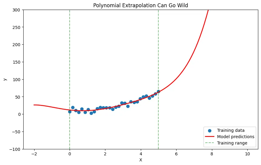
Solution: Never trust polynomial predictions far outside your training data range.

4. Choosing the Wrong Transformation

Problem: Forcing polynomial fit on exponential data, or vice versa.

# Exponential data with multiplicative noise
np.random.seed(42)
X = np.linspace(0, 5, 50).reshape(-1, 1)
y = 2 * np.exp(0.8 * X.squeeze()) * np.exp(np.random.randn(50) * 0.2)

# Wrong: polynomial fit
poly_model = make_pipeline(
    PolynomialFeatures(degree=3),
    LinearRegression()
)
poly_model.fit(X, y)
poly_pred = poly_model.predict(X)
poly_r2 = r2_score(y, poly_pred)

# Right: exponential fit
exp_model = LinearRegression()
exp_model.fit(X, np.log(y))
exp_pred = np.exp(exp_model.predict(X))
exp_r2 = r2_score(y, exp_pred)

print(f"Polynomial R²: {poly_r2:.3f}")
print(f"Exponential R²: {exp_r2:.3f}")

Output:

Polynomial R²: 0.936
Exponential R²: 0.934

Solution: Plot your data and hypothesize the relationship type before choosing a model.

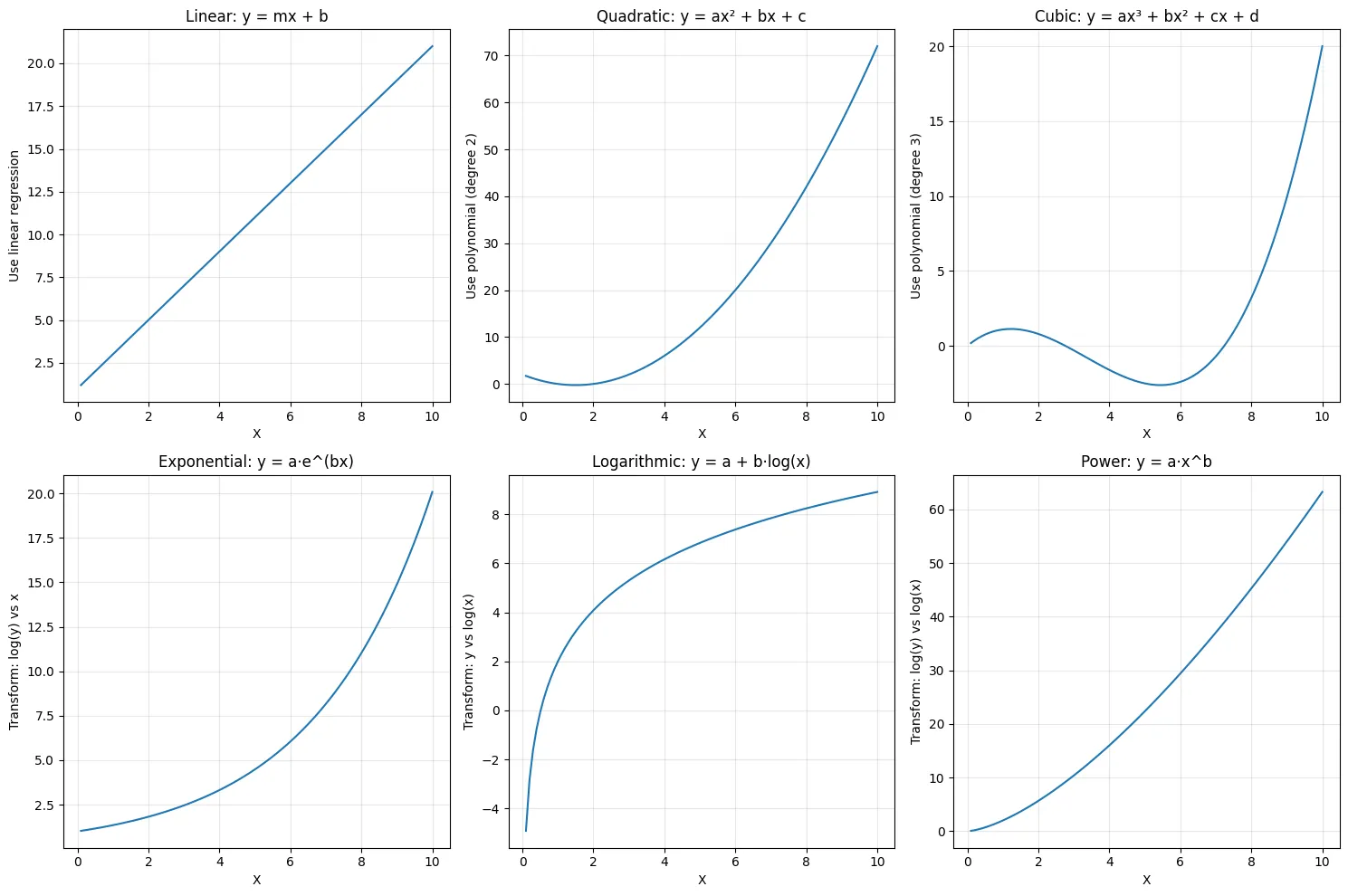
Choosing the Right Non-Linear Model

Decision Framework

import matplotlib.pyplot as plt
import numpy as np

def plot_relationship_types():
    """Visualize different relationship types"""
    X = np.linspace(0.1, 10, 100)
    
    fig, axes = plt.subplots(2, 3, figsize=(15, 10))
    
    # Linear
    axes[0, 0].plot(X, 2*X + 1)
    axes[0, 0].set_title('Linear: y = mx + b')
    axes[0, 0].set_ylabel('Use linear regression')
    
    # Polynomial (quadratic)
    axes[0, 1].plot(X, X**2 - 3*X + 2)
    axes[0, 1].set_title('Quadratic: y = ax² + bx + c')
    axes[0, 1].set_ylabel('Use polynomial (degree 2)')
    
    # Polynomial (cubic)
    axes[0, 2].plot(X, 0.1*X**3 - X**2 + 2*X)
    axes[0, 2].set_title('Cubic: y = ax³ + bx² + cx + d')
    axes[0, 2].set_ylabel('Use polynomial (degree 3)')
    
    # Exponential
    axes[1, 0].plot(X, np.exp(0.3*X))
    axes[1, 0].set_title('Exponential: y = a·e^(bx)')
    axes[1, 0].set_ylabel('Transform: log(y) vs x')
    
    # Logarithmic
    axes[1, 1].plot(X, 2 + 3*np.log(X))
    axes[1, 1].set_title('Logarithmic: y = a + b·log(x)')
    axes[1, 1].set_ylabel('Transform: y vs log(x)')
    
    # Power law
    axes[1, 2].plot(X, 2 * X**1.5)
    axes[1, 2].set_title('Power: y = a·x^b')
    axes[1, 2].set_ylabel('Transform: log(y) vs log(x)')
    
    for ax in axes.flat:
        ax.grid(True, alpha=0.3)
        ax.set_xlabel('X')
    
    plt.tight_layout()
    plt.show()

plot_relationship_types()

Output:

Step-by-Step Process

1. Plot your data: Look for patterns visually
2. Identify the curve type: Does it accelerate, decelerate, or oscillate?
3. Start simple: Try polynomial degree 2 first
4. Check diagnostics: Look at residual plots and R² scores
5. Compare models: Test multiple approaches with cross-validation
6. Validate: Always test on held-out data

Practical Comparison Example

from sklearn.metrics import mean_squared_error, r2_score
from sklearn.model_selection import cross_val_score

# Generate data (true relationship is quadratic)
np.random.seed(42)
X = np.linspace(1, 10, 100).reshape(-1, 1)
y = 5 + 3*X.squeeze() - 0.5*X.squeeze()**2 + np.random.randn(100) * 5

# Compare different models
models = {
    'Linear': LinearRegression(),
    'Polynomial (degree 2)': make_pipeline(PolynomialFeatures(2), LinearRegression()),
    'Polynomial (degree 3)': make_pipeline(PolynomialFeatures(3), LinearRegression()),
    'Logarithmic': None  # Will handle separately
}

results = {}

for name, model in models.items():
    if model is not None:
        # Cross-validation
        cv_scores = cross_val_score(model, X, y, cv=5, 
                                     scoring='neg_mean_squared_error')
        results[name] = -cv_scores.mean()

# Logarithmic model (transform features)
log_model = LinearRegression()
cv_scores_log = cross_val_score(log_model, np.log(X), y, cv=5,
                                scoring='neg_mean_squared_error')
results['Logarithmic'] = -cv_scores_log.mean()

# Print results
print("Cross-Validation MSE:")
for name, mse in sorted(results.items(), key=lambda x: x[1]):
    print(f"  {name:.<30} {mse:>10.2f}")

Output:

Cross-Validation MSE:
  Polynomial (degree 2).........      23.05
  Polynomial (degree 3).........      36.12
  Linear........................      52.45
  Logarithmic...................     104.78

When to Use Polynomial vs Other Non-Linear Models

Use Polynomial Regression When:

• Relationship has clear curvature with turning points
• You need interpretability (degree 2-3 is still understandable)
• Data range is limited (polynomial doesn’t need to extrapolate)
• You have enough data to support higher degrees
• Quick baseline is needed

Use Exponential/Logarithmic When:

• Growth/decay patterns are present
• Relationship spans several orders of magnitude
• Domain knowledge suggests specific functional form
• Data shows compounding or saturation effects

Consider Other Methods When:

• Multiple different curve types in same dataset → Tree-based models
• Very complex patterns → Neural networks, GAMs
• Need maximum interpretability → Keep it simple with degree 2 polynomial
• Have categorical features → Use more flexible methods

Real-World Example: Complete Workflow

import pandas as pd
from sklearn.model_selection import train_test_split
from sklearn.preprocessing import StandardScaler
from sklearn.pipeline import make_pipeline
from sklearn.linear_model import Ridge

# Load sample data (or create your own)
np.random.seed(42)
data = pd.DataFrame({
    'experience': np.random.uniform(0, 20, 200),
    'education': np.random.uniform(12, 20, 200),
    'age': np.random.uniform(22, 65, 200)
})

# Non-linear salary relationship
data['salary'] = (
    30000 + 
    2000 * data['experience'] + 
    100 * data['experience']**2 +
    3000 * data['education'] +
    500 * data['age'] -
    5 * data['age']**2 +
    np.random.randn(200) * 5000
)

# Split data
X = data[['experience', 'education', 'age']]
y = data['salary']
X_train, X_test, y_train, y_test = train_test_split(X, y, test_size=0.2, random_state=42)

# Build pipeline with polynomial features and regularization
model = make_pipeline(
    StandardScaler(),
    PolynomialFeatures(degree=2, include_bias=False),
    Ridge(alpha=10)  # Regularization to prevent overfitting
)

# Train model
model.fit(X_train, y_train)

# Evaluate
train_score = model.score(X_train, y_train)
test_score = model.score(X_test, y_test)

print(f"Training R²: {train_score:.3f}")
print(f"Test R²: {test_score:.3f}")

# Make prediction
new_person = pd.DataFrame({
    'experience': [5],
    'education': [16],
    'age': [30]
})
predicted_salary = model.predict(new_person)
print(f"\nPredicted salary: ${predicted_salary[0]:,.0f}")

# Analyze feature importance (approximate)
poly_features = model.named_steps['polynomialfeatures']
feature_names = poly_features.get_feature_names_out(['experience', 'education', 'age'])
coefficients = model.named_steps['ridge'].coef_

# Top 5 important features
importance_df = pd.DataFrame({
    'feature': feature_names,
    'coefficient': np.abs(coefficients)
}).sort_values('coefficient', ascending=False)

print("\nTop 5 most important features:")
print(importance_df.head())

Output:

Training R²: 0.954
Test R²: 0.961

Predicted salary: $102,766

Top 5 most important features:
         feature   coefficient
0     experience  21415.527514
1      education   6203.021220
3   experience^2   2972.191127
2            age   1185.991003
7  education age    913.210335

Next Steps

Once you’re comfortable with polynomial and non-linear regression, consider these extensions:

Regularized Polynomial Regression

from sklearn.linear_model import Ridge, Lasso

# Ridge regression with polynomial features
model = make_pipeline(
    StandardScaler(),
    PolynomialFeatures(degree=3),
    Ridge(alpha=1.0)  # L2 regularization
)

# Lasso for feature selection
model = make_pipeline(
    StandardScaler(),
    PolynomialFeatures(degree=3),
    Lasso(alpha=1.0)  # L1 regularization, some coefficients become 0
)

Generalized Additive Models (GAMs)

For even more flexibility with interpretability, explore GAMs which fit smooth curves to each feature separately.

Advanced Methods

• Splines: Piecewise polynomial functions
• Kernel methods: SVM with non-linear kernels
• Tree-based models: Random Forest, XGBoost (handle non-linearity automatically)
• Neural networks: For highly complex non-linear patterns

Key Takeaways

1. Always visualize first: Plot your data to understand its shape
2. Start simple: Try polynomial degree 2 before going higher
3. Use cross-validation: Prevent overfitting with proper validation
4. Scale your features: Critical for polynomial regression
5. Don’t extrapolate: Polynomial models are unreliable outside training range
6. Consider domain knowledge: Sometimes exponential or logarithmic makes more sense
7. Balance complexity: More complex isn’t always better

Polynomial and non-linear regression bridge the gap between simple linear models and complex machine learning algorithms. Master these techniques, and you’ll be able to model most real-world relationships while maintaining interpretability and computational efficiency.